
You come across a sports car racing a jeep on the highway. Who do you think loses? The jeep, of course, but as soon as you move to rocky terrain, the outcome is the opposite. It doesn’t matter how fancy the car is; if it’s not the right one for the job, it doesn’t work. Machine learning works the same way; there’s no single best approach, only a specific method that fits the shape of the problem in front of it. The whole point of machine learning is to train the machine using that specific approach to go through thousands of data points and find the patterns instead of doing it manually.
To see why that actually matters, look at the numbers. Thinking about climate change, we often picture planes and jet engines with huge emissions, but the fact is that aviation accounts for only 3% of global greenhouse gas emissions, whereas, in comparison, buildings and construction account for 34%.
The way we design and construct our buildings is a massive lever on how the emissions are impacted; buildings leak energy like water through a sieve, and hitting our decarbonization goals means finding better ways to plug that leak.
The leak shows up in the form of heating and cooling load. Higher energy needs for heating or cooling the building means more energy gets burned to keep people comfortable which increases the GHG emissions tied to those buildings. Get the load values down, and you cut emissions at the source before a single brick is laid.
For this ML Explainer, I used the Energy Efficiency dataset, which contains 768 different building shapes, all simulated with eight varying features like roof area, height, and orientation. My goal is to predict those two loads directly from these features.
The method
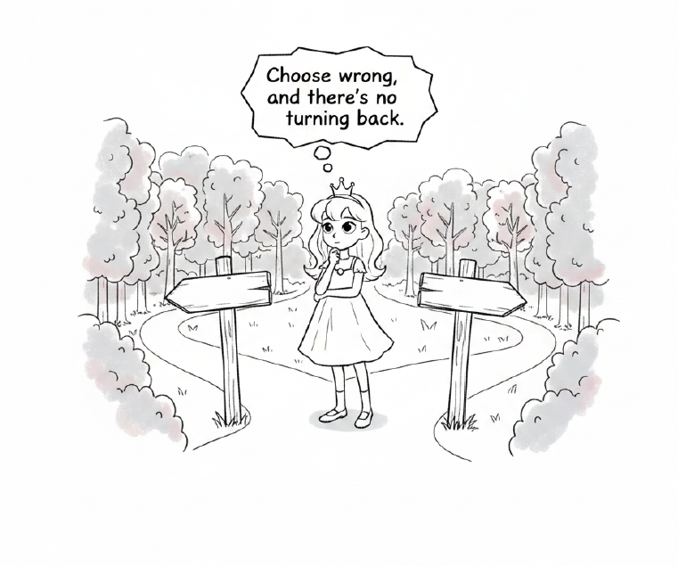
Consider yourself on a road, a fork sign says turn left for blueberries and right for raspberries. You pick one, walk further, and hit another fork, right leads to big blueberries, left leads to smaller ones. This keeps happening, fork after fork, size, ripeness, weight, until you move from a few scattered trees into a dense forest, and at the end of the path, you arrive at the exact berry with the exact features you were looking for. That’s a decision tree.
There are a couple of things worth knowing about this method. You can’t go back on the path that you have chosen. Once you turn left at a fork, you never find out what was down the right path, even if the right path would have led somewhere better. That’s what makes the model decisive but also risky. One bad fork early on can send you confidently down the wrong path for the rest of the walk.
Second thing to note is that this method works best with non-linear relationships. Consider the case of heating water in a kettle, the temperature climbs proportionally, but right at 100°C, it stops increasing and instead turns to steam.
That sudden, irregular jump in its state is non-linearity. And it’s exactly what a fork in the road is built to catch. Every fork in this method is a single yes or no question. It doesn’t care about smooth, steady change; it only cares about finding the one exact point where everything flips. Give the model a numeric relationship between its features, and it doesn’t need a complicated formula to describe the whole curve; it just needs to find that one “click” point.
The Problem with One Path
But here’s the catch: if the model is built on just one decision tree, it will build a perfect map for every single berry it has already seen, memorizing that exact path down to the last detail. If you try to use this to find berries in different locations, you will probably end up in a bear cave.
Overfitting occurs when the model learns too much from the data, to the point that it fails to recognize the unseen data. To fix this, we stop the tree from overgrowing. This is done by testing a bunch of different tree sizes. I found that capping the tree at exactly 50 “leaf nodes,” the final destinations at the end of the forks, gave the most accurate predictions. With this trimmed tree, the model’s error rate, which shows how far off its prediction was from the actual energy load, dropped to 0.38 for heating and 1.39 for cooling.
Can we further improve the model?
Imagine instead of just sending one person, like in our previous analogy, we send groups of people from different entry points. Each person gets a different part of the same map and looks at different berries. When they all come back to the edge of the forest, we average out their guesses.
A Random Forest algorithm works on this exact principle. It builds a literal “forest” of many individual decision trees, feeds them slightly randomized views of the data, and lets them vote on the final prediction. In my model, the forest model reduced the error for predicting the heating load from 0.38 down to 0.35, and the cooling load error dropped from 1.39 to 1.18. The crowd beat the individual.
One thing to note is that there’s no considerable reduction in the error because my trained model is already doing a good job at predicting the load values; but as a general rule of thumb, the random forest model outperforms decision trees by a notable amount when the overfitting is large (minimal value in this case).
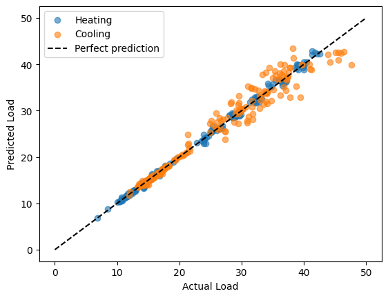
Figure 1: A quick check to see if the predicted load values are correct
Model insights decoded
By studying the random forest, I determined which of the eight building traits actually drove the results. In the world of machine learning, we call this Feature Importance.
I bet on the orientation feature of the building, thinking it was an important driver because, intuitively, receiving more direct sunlight implies more warming. I was completely wrong. The algorithm discovered that Orientation (X6) was the least significant factor of all.
It turns out, the real heavyweights are far more structural. Relative Compactness (X1), which is essentially how tightly packed the building’s volume is, and Overall Height (X5) are the ones that drive the prediction for cooling load.
Similarly, for heating load, Relative Compactness (X1) and Surface Area (X2) drove the results.
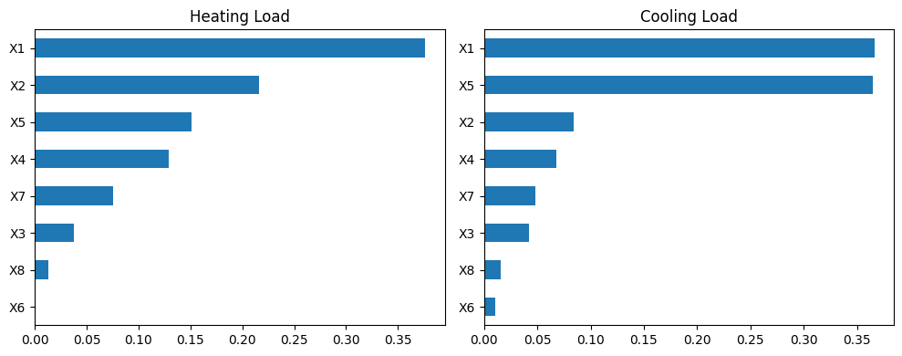
Figure 2: Feature Importance map showing who drives the predictions
This is an important result because now we can calculate a building’s thermal footprint before the shovel even hits the ground, transforming that staggering 34% emissions hurdle into a challenge we can fundamentally out-engineer through smarter design.
The ML explainer’s results are derived from training my model on the dataset created by Angeliki Xifara (Civil/Structural Engineer) which was processed by Athanasios Tsanas (Oxford Centre for Industrial and Applied Mathematics, University of Oxford, UK).
You can find the dataset at : https://www.kaggle.com/datasets/elikplim/eergy-efficiency-dataset